Quick cholesteric tutorial

In this section aimed at users who are not experienced in programming and/or in Python, we explain a code minimal working example to:

• create a cholesteric architecture with a chosen pitch, tilt and handedness
• obtain a 3D representation of the cholesteric architecture
• calculate the reflectance in transmittance in the circular polarisation basis for a chosen angle of incidence
• extract and plot the results in Python
• export the results for further processing in MATLAB

First, the user must import the required packages. We need PyLLama for the optical calculations, Cholesteric to create the cholesteric architecture, NumPy for basic numerical calculation and Matplotlib.PyPlot for plotting. In Python, all packages are imported in lowercaps at the beginning of the code and they are often given a shorter name (ch instead of cholesteric for example).

# Import the required packages
import pyllama as ll
import cholesteric as ch
import numpy as np
import matplotlib.pyplot as plt

Then, the user creates their Cholesteric object with ch.Cholesteric:

# Cholesteric object
pitch_nm = 500
tilt_rad = 10 * np.pi / 180
chole = ch.Cholesteric(pitch360=pitch_nm,
                       tilt_rad=tilt_rad,
                       handedness=1)

The user can obtain a 3D representation of the Cholesteric object with the function plot_simple(). The view parameters defines the viewing angle and the type parameters defines how the pseudolayers are represented (here, with arrows). The user should note that the , and axes might not have exactly the same scale.

# 3D representation of the cholesteric object
fig_3D, ax_3D = chole.plot_simple(view="classic", type="arrow")

The user can then define the incident conditions upon the cholesteric and obtain their 3D representation. When the cholesteric is tilted, the axis will be shifted to the helical axis for the calculations.

# Incident conditions and 3D representation
theta_in_deg = 50
theta_in_rad = theta_in_deg * np.pi / 180
chole.plot_add_optics(fig_3D, ax_3D, theta_in_rad)

The output is displayed on Figure Fig. 2.

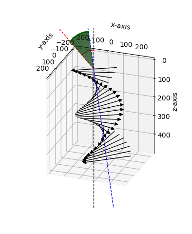
Fig. 2 3D representation of chole obtained with the functions plot_simple() and add_optics().

Then, the user can choose the optical parameters such as the average refractive index and the birefringence, and create a Spectrum object:

# Optical parameters
n_av = 1.433
biref = 0.04
n_e = n_av + 0.5 * biref
n_o = n_av - 0.5 * biref
n_entry = n_av
n_exit = n_av
N_per = 20
wl_nm_list = np.arange(400, 800)

# Creation of the spectrum
spectrum = ll.Spectrum(wl_nm_list,
                       "CholestericModel",
                       dict(chole=chole,
                            n_e=n_e,
                            n_o=n_o,
                            n_entry=n_entry,
                            n_exit=n_exit,
                            N_per=N_per,
                            theta_in_rad=theta_in_rad))

The calculation of the reflectance and transmittance is done in one go; the parameter circ=True enables to calculate the reflectance and transmittance in the circular polarisation basis, the parameter method="SM" enables to choose the always-accurate scattering matrix method for the calculation and the parameter talk=True allows do display the calculation progress on the screen. The spectrum will take about 30 seconds to be calculated.

# Calculation of the reflectance and transmittance
spectrum.calculate_refl_trans(circ=True, method="SM", talk=True)

The results can be plotted:

# Plot the spectra
fig = plt.figure()

ax1 = fig.add_subplot(311)
ax1.plot(wl_nm_list, spectrum.data['R_R_to_R'], label="RCP to RCP")
ax1.plot(wl_nm_list, spectrum.data['R_R_to_L'], label="RCP to LCP")
plt.legend(loc=2)
plt.xlim([400, 800])
plt.ylim([0, 1])
plt.xlabel('Wavelength (nm)')
plt.ylabel('Reflectance')
ax1.set_title('Incoming RCP')

ax2 = fig.add_subplot(312)
ax2.plot(wl_nm_list, spectrum.data['R_L_to_R'], label="LCP to RCP")
ax2.plot(wl_nm_list, spectrum.data['R_L_to_L'], label="LCP to LCP")
plt.legend(loc=2)
plt.xlim([400, 800])
plt.ylim([0, 1])
plt.xlabel('Wavelength (nm)')
plt.ylabel('Reflectance')
ax2.set_title('Incoming LCP')

For incoming unpolarised light, the user should not forget to average the incoming RCP and incoming LCP:

ax3 = fig.add_subplot(313)
ax3.plot(wl_nm_list, 0.5 * (spectrum.data['R_R_to_R']
                            + spectrum.data['R_R_to_L']
                            + spectrum.data['R_L_to_R']
                            + spectrum.data['R_L_to_L']),
                            label="reflection")
ax3.plot(wl_nm_list, 0.5 * (spectrum.data['T_R_to_R']
                            + spectrum.data['T_R_to_L']
                            + spectrum.data['T_L_to_R']
                            + spectrum.data['T_L_to_L']),
                            label="transmission")
plt.legend(loc=2)
plt.xlim([400, 800])
plt.ylim([0, 1])
plt.xlabel('Wavelength (nm)')
plt.ylabel('Intensity')
ax3.set_title('Incoming unpolarised')

The user can make the layout of the plots a bit nicer, before saving and displaying the figure (without plt.show(), the plots will not be shown on the computer screen):

plt.tight_layout()
fig.savefig("script_cholesteric_example.png", dpi=300)
plt.show()

The output is displayed on Figure Fig. 3.

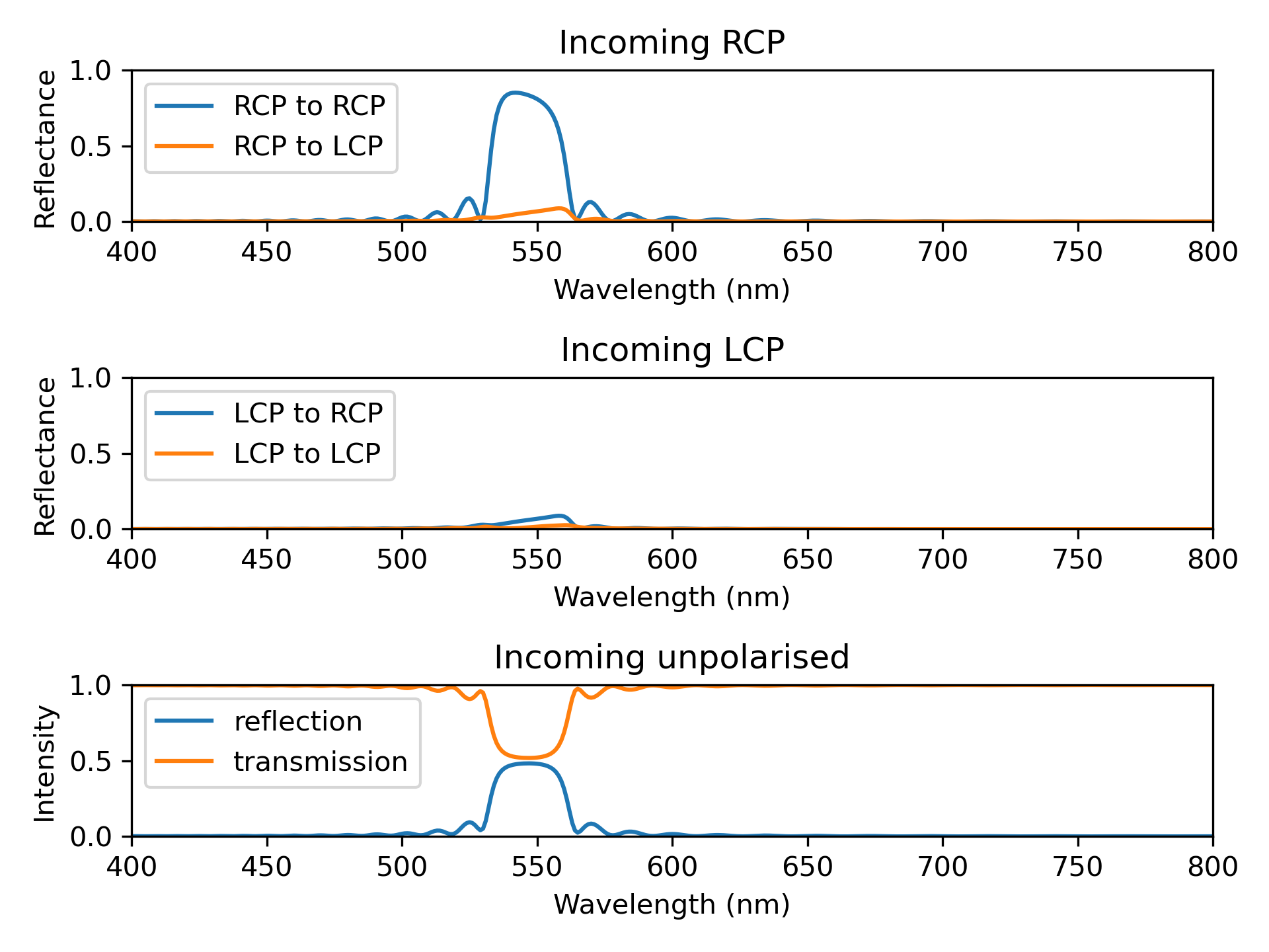
Fig. 3 Spectra obtained with the Spectrum and CholestericModel.

The results can be exported to MATLAB very simply for further processing. The parameters such as the refractive indices are also exported, as well as all the fields of the cholesteric object (such as the directors of the pseudo-layers). To export with Pickles (for Python further processing), the user should replace the extension .mat by .pck.

# Export the spectra to an external file
path_out = "pyllama_cholesteric_spectrum.mat"
spectrum.export(path_out)