Calculating the reflection and transmission spectra of a stack¶

The section Creating a multilayer stack explains how to create the multilayer stack with three methods, which all enable to calculate the reflection and transmission spectra of the stack with different level of additional details:

creating a multilayer stack from scratch with the classes Structure Layer, and working directly with classes that handle the optical calculations. This method gives direct access to the partial waves inside each layer of the multilayer stack, to the transfer and scattering matrices, to the multilayer stack’s reflection and transmission coefficients and to the multilayer stack’s reflectance and transmittance for one wavelength.
creating multilayer stacks with the abstract class Model and its children, and writing one’s own child class when a different kind of stack is needed. This method gives direct access to the multilayer stack’s reflectance and transmittance for one wavelength. Additionally, the layer’s partial waves, the transfer and scattering matrices and the reflection and transmission coefficients can also be obtained since the Model creates a Structure.
using the class Spectrum that provides a higher level of automation. This method gives direct access to the multilayer stack’s reflectance and transmittance for a range of wavelength.

This section explains how to get the reflection spectrum of a multilayer stack which has been created through one of there three methods, following the tutorials Creating a multilayer stack.

From scratch: the technical way¶

When the user follows the method “from scratch” with the class Structure to create a multilayer stack my_stack_structure, they interact directly with the classes that handle the optics calculation. The Structure that represents the multilayer stack contains a list of Layers and the entry and exit HalfSpaces (which are children of Layer). Layers and HalfSpaces implement the calculation of Berreman’s matrix and of the layer’s eigenvalues and eigenvectors, used to calculate the layer’s partial waves. These are calculated immediately upon the creation of the Layer or HalfSpace and can be accessed through:

my_stack_structure.layers[k].D                # layer’s Berreman’s matrix
my_stack_structure.layers[k].eigenvalues      # layer’s eigenvalues
my_stack_structure.layers[k].eigenvectors     # layer’s eigenvectors
my_stack_structure.layers[k].partial_waves    # layer’s partial waves

where k is the index of the Layer in the Structure my_stack_structure.

A Structure therefore automatically contains a series of four partial waves per layer, which are used to construct its transfer matrix or its scattering matrix (for the wavelength that was used to create the Structure). The transfer and scattering matrices can be calculated the following way:

my_stack_structure.build_transfer_matrix()    # transfer matrix
my_stack_structure.build_scattering_matrix()  # scattering matrix

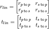
Reflection and transmission coefficients in the linear polarisation basis (for the wavelength that was used to create the Structure) can be calculated with:

J_refl_lin, J_trans_lin = my_stack_structure.get_fresnel()

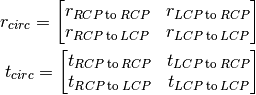
and converted to the circular polarisation basis with:

J_refl_circ, J_trans_circ = Structure.fresnel_to_fresnel_circ(J_lin)

The results are two $2\times2$ Numpy arrays of reflection coefficients ( $r$ ) and transmission coefficients ( $t$ ) organised the following way:

in the linear polarisation basis:

$r_{lin} = \begin{bmatrix} r_{p \: \text{to} \: p} & r_{s \: \text{to} \: p} \\ r_{p \: \text{to} \: s} & r_{s \: \text{to} \: s} \end{bmatrix} t_{lin} = \begin{bmatrix} t_{p \: \text{to} \: p} & t_{s \: \text{to} \: p} \\ t_{p \: \text{to} \: s} & t_{s \: \text{to} \: s} \end{bmatrix}$
in the circular polarisation basis:

$r_{circ} = \begin{bmatrix} r_{RCP \: \text{to} \: RCP} & r_{LCP \: \text{to} \: RCP} \\ r_{RCP \: \text{to} \: LCP} & r_{LCP \: \text{to} \: LCP} \end{bmatrix} t_{circ} = \begin{bmatrix} t_{RCP \: \text{to} \: RCP} & t_{LCP \: \text{to} \: RCP} \\ t_{RCP \: \text{to} \: LCP} & t_{LCP \: \text{to} \: LCP} \end{bmatrix}$

For example, the user can access the reflection coefficient for incoming s-polarised light reflected as p-polarised light of the multilayer stack represented by the Structure my_stack_structure with:

J_lin, _ = my_stack_structure.get_fresnel()
J_lin[0, 1]

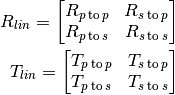
The reflectance and transmittance of the multilayer stack (for the wavelength that was used to create the Structure) can be obtained with:

my_stack_structure.get_refl_trans(circ=<False|True>, method=<"SM"|"TM">)

where method defines the matrix method used ("SM" (default) for the scattering matrix method and "TM" for the transfer matrix method) and circ=False (default) calculates the reflectance and transmittance in the linear polarisation basis and circ=True calculates them in the circular polarisation basis.

The results are two $2\times2$ Numpy arrays of reflectances ( $R$ ) organised the following way:

in the linear polarisation basis:

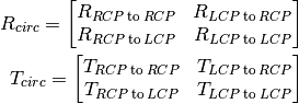
$R_{lin} = \begin{bmatrix} R_{p \: \text{to} \: p} & R_{s \: \text{to} \: p} \\ R_{p \: \text{to} \: s} & R_{s \: \text{to} \: s} \end{bmatrix} T_{lin} = \begin{bmatrix} T_{p \: \text{to} \: p} & T_{s \: \text{to} \: p} \\ T_{p \: \text{to} \: s} & T_{s \: \text{to} \: s} \end{bmatrix}$
in the circular polarisation basis:

$R_{circ} = \begin{bmatrix} R_{RCP \: \text{to} \: RCP} & R_{LCP \: \text{to} \: RCP} \\ R_{RCP \: \text{to} \: LCP} & R_{LCP \: \text{to} \: LCP} \end{bmatrix} T_{circ} = \begin{bmatrix} T_{RCP \: \text{to} \: RCP} & T_{LCP \: \text{to} \: RCP} \\ T_{RCP \: \text{to} \: LCP} & T_{LCP \: \text{to} \: LCP} \end{bmatrix}$

To calculate the reflection and transmission spectra of the stack over a range of wavelengths, the user must create a new Structure for each wavelength and recalculate the reflectance, for example with:

# Creation of an empty variable
reflection_s_to_p = []

# Creation of the wavelengths
wl_nm_list = range(400, 800)

# Calculation of the reflectance for each wavelength
for wl_nm in wl_nm_list:
    # Calculation of the wavevector
    k0 = 2 * numpy.pi / wl_nm
    Kx = n_entry * numpy.sin(theta_in_rad)
    Ky = 0
    Kz_entry = n_entry * numpy.cos(theta_in_rad)
    theta_out_rad = numpy.arcsin((n_entry / n_exit) * numpy.sin(self.theta_in_rad))
    Kz_exit = n_exit * numpy.cos(theta_out_rad)

    # Creation of the entry and exit half-spaces and of the two layers
    entry = HalfSpace(epsilon_entry, Kx, Kz_entry, k0)
    exit = HalfSpace(epsilon_exit, Kx, Kz_exit, k0)
    layer_a = Layer(eps_a, thick_a, Kx, k0)
    layer_b = Layer(eps_b, thick_b, Kx, k0)

    # Creation of the periodic stack
    my_stack_structure = Structure(entry, exit, Kx, Ky, Kz_entry, Kz_exit, k0)
    my_stack_structure.add_layers([layer_a, layer_b])
    my_stack_structure.N_periods = N

    # Calculation of the reflectance and storage
    J_refl_lin, _ = my_stack_structure.get_refl_trans()
    reflection_s_to_p.append(J_refl_lin[0, 1])

# Plotting
matplotlib.pyplot.plot(wl_nm_list, reflection_s_to_p)

where:

eps_a and eps_b are the permittivity tensors (3x3 Numpy array) of the layer, which can represent a material that is isotropic or anisotropic, absorbing or non-absorbing
thick_a and thick_b are the thicknesses of the two layers of the periodic pattern, in nanometers
N is the number of periods
`` theta_in_rad`` is the angle of incidence upon the stack, in radians
eps_entry and eps_exit are the permittivities of the two isotropic half-spaces; they can be defined differently for each wavelength if the materials are dispersive

With the `Model` class: the flexible way¶

When the user creates a multilayer stack my_stack_model through one of the Model children classes, the reflectance and transmittance of the multilayer stack (for the wavelength that was used to create the Structure) can be obtained with:

my_stack_model.get_refl_trans(circ=<False|True>, method=<"SM"|"TM">)

where method defines the matrix method used ("SM" (default) for the scattering matrix method and "TM" for the transfer matrix method) and circ=False (default) calculates the reflectance and transmittance in the linear polarisation basis and circ=True calculates them in the circular polarisation basis.

The results are two $2\times2$ Numpy arrays of reflectances ( $R$ ) organised the following way:

in the linear polarisation basis:

$R_{lin} = \begin{bmatrix} R_{p \: \text{to} \: p} & R_{s \: \text{to} \: p} \\ R_{p \: \text{to} \: s} & R_{s \: \text{to} \: s} \end{bmatrix} T_{lin} = \begin{bmatrix} T_{p \: \text{to} \: p} & T_{s \: \text{to} \: p} \\ T_{p \: \text{to} \: s} & T_{s \: \text{to} \: s} \end{bmatrix}$
in the circular polarisation basis:

$R_{circ} = \begin{bmatrix} R_{RCP \: \text{to} \: RCP} & R_{LCP \: \text{to} \: RCP} \\ R_{RCP \: \text{to} \: LCP} & R_{LCP \: \text{to} \: LCP} \end{bmatrix} T_{circ} = \begin{bmatrix} T_{RCP \: \text{to} \: RCP} & T_{LCP \: \text{to} \: RCP} \\ T_{RCP \: \text{to} \: LCP} & T_{LCP \: \text{to} \: LCP} \end{bmatrix}$

Note

Each children class of Model contains a Structure that can be accessed through my_stack_model.structure and the the previous part of this tutorial can be applied to my_stack_model.structure to access the partial waves, the transfer or scattering matrices and the reflection and transmission coefficients.

To calculate the reflection and transmission spectra of the stack over a range of wavelengths, the user must create a new Model for each wavelength and recalculate the reflectance and transmittance, for example with:

# Creation of an empty variable
reflection_s_to_p = []

# Creation of the wavelengths
wl_nm_list = range(400, 800)

# Calculation of the reflectance for each wavelength
for wl_nm in wl_nm_list:
    # Creation of the periodic stack
    my_stack_model = StackModel([eps_a, eps_b],
                                [thick_a, thick_b],
                                n_entry,
                                n_exit,
                                wl_nm,
                                theta_in_rad,
                                N)

    # Calculation of the reflectance and storage
    J_refl_lin, _ = my_stack_model.get_refl_trans()
    reflection_s_to_p.append(J_refl_lin[0, 1])

# Plotting
matplotlib.pyplot.plot(wl_nm_list, reflection_s_to_p)

where:

eps_a and eps_b are the permittivity tensors (3x3 Numpy array) of the layer, which can represent a material that is isotropic or anisotropic, absorbing or non-absorbing
thick_a and thick_b are the thicknesses of the two layers of the periodic pattern, in nanometers
N is the number of periods
`` theta_in_rad`` is the angle of incidence upon the stack, in radians
n_entry and n_exit are the refractive indices of the two isotropic half-spaces; they can be defined differently for each wavelength if the materials are dispersive

With the `Spectrum` class: the automated way¶

When the user creates a multilayer stack my_stack_spec through the Spectrum class, the reflection and transmission spectra of the multilayer stack (for the range of wavelength that was inputted in the Spectrum) can be obtained with:

my_stack_spectrum.calculate_refl_trans(circ=<False|True>, method=<"SM"|"TM">, talk=<False|True>)

where method defines the matrix method used ("SM" (default) for the scattering matrix method and "TM" for the transfer matrix method), circ=False (default) calculates the reflectance and transmittance in the linear polarisation basis and circ=True calculates them in the circular polarisation basis, and talk=True enables to display the calculation progress on the screen (default is False).

The calculated reflection spectra are stored into the dictionary my_stack_spectrum.data and can be accessed with:

in the linear polarisation basis: my_stack_spectrum.data["R_p_to_p_to_p"], my_stack_spectrum.data["R_s_to_p"], my_stack_spectrum.data["R_p_to_s"], my_stack_spectrum.data["R_s_to_s"]
in the circular polarisation basis: my_stack_spectrum.data["R_R_to_R"], my_stack_spectrum.data["R_L_to_R"], my_stack_spectrum.data["R_R_to_L"], my_stack_spectrum.data["R_L_to_L"]

and similarly for the transmission spectra: - in the linear polarisation basis: my_stack_spectrum.data["T_p_to_p"], my_stack_spectrum.data["T_s_to_p"], my_stack_spectrum.data["T_p_to_s"], my_stack_spectrum.data["T_s_to_s"]

in the circular polarisation basis: my_stack_spectrum.data["T_R_to_R"], my_stack_spectrum.data["T_L_to_R"], my_stack_spectrum.data["T_R_to_L"], my_stack_spectrum.data["T_L_to_L"]

The calculated spectra (everything stored in my_stack_spectrum.data) can then be exported in MATLAB or Python-compatible format with:

my_stack_spectrum.export(path_out, with_param=<True|False>)

where:

path_out is the name of the file. If it ends with .mat, the export will be in MATLAB-compatible format, and if it ends with .pck, the export will be in Python-compatible format (with Pickles)
with_param is set to True (default) when the parameters user for the model are exported too and to False when they are not exported

Note

Some Models may take as input parameters objects that are created through the user’s custom-made libraries (for example, CholestericModel requires an instance of a Cholesteric as a parameter). These objects will be stored in the Model’s parameters. MATLAB can import any unknown object in shape of MATLAB’s type struct but Python can only import objects for whose it can load the libraries that created them. In this case, exporting the spectra without the parameters may be useful, but this is not the default option.

The calculation the reflection spectrum of the stack over a range of wavelengths is automatic, for example with:

# Creation of the wavelengths
wl_nm_list = range(400, 800)

# Parameters for the stack
model_type = "StackModel"
model_parameters = {"eps_list": [eps_a, eps_b],
                    "thickness_nm_list": [thick_a, thick_b],
                    "n_entry": n_entry,
                    "n_exit": n_exit,
                    "theta_in_rad": theta_in_rad,
                    "N_per": N}

# Creation of the periodic stack
my_stack_spec = Spectrum(wl_nm_list, model_type, model_parameters)

# Calculation of the reflectance spectrum in one go
my_stack_spec.calculate_refl_trans()

# Plotting
matplotlip.pyplot.plot(wl_nm_list, my_stack_spec.data["R_s_to_p"])

# Export for MATLAB
    # All polarisation combinations are exported (p to p, s to p, p to p, s to s)
my_stack_spec.export("my_file_name.mat")

where:

eps_a and eps_b are the permittivity tensors (3x3 Numpy array) of the layer, which can represent a material that is isotropic or anisotropic, absorbing or non-absorbing; if the material is dispersive, a Model different than StackModel must be used that is able to handle a list of permittivities
thick_a and thick_b are the thicknesses of the two layers of the periodic pattern, in nanometers
N is the number of periods
theta_in_rad is the angle of incidence upon the stack, in radians
n_entry and n_exit are the refractive indices of the two isotropic half-spaces; they can be defined differently for each wavelength if the materials are dispersive

Calculating the reflection and transmission spectra of a stack¶

From scratch: the technical way¶

With the Model class: the flexible way¶

With the Spectrum class: the automated way¶

With the `Model` class: the flexible way¶

With the `Spectrum` class: the automated way¶