Choosing which matrix method to use
Note
The theory that leads to the equations presented in this section is detailed in “PyLlama: a stable and flexible Python toolkit for the electromagnetic modeling of multilayered anisotropic media” (in preparation).
The transfer matrix and the scattering matrix both link the incoming, reflected and transmitted electric fields, but their equations are built differently. The notations are displayed on Figure Fig. 4.
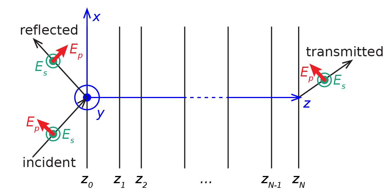
Fig. 4 Schematic of the electric field direction for  and
and  -polarisations.
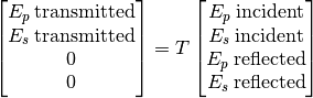
The transfer matrix equation is:
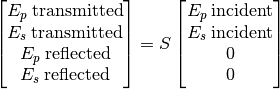
and the scattering matrix equation is:
The reflection and transmission coefficients are extracted from either of these matrix equations to obtain:
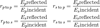
and:
Mathematically, both equations lead to the same result and choosing which one to use has no impact on the reflection and transmission coefficients, but numerically, differences can be observed in the robustness and in the computation time.
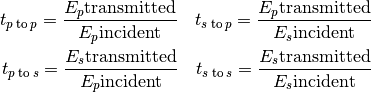
As an example, we built two cholesterics with a different birefringence (chole_1 with  and
and chole_2 with  ) and a different number of periods (20 for
 chole_1 and 200 for chole_2), and confronted the transfer and scattering matrix methods. A we can see on Figure Fig. 5, the two matrix methods give the exact same results when the birefringence is low and when the number of periods is low. However, for a higher birefringence and a larger number of periods, the transfer matrix (be it calculated with the eigenvalues and eigenvectors or with the direct exponential of Berreman’s matrix) is numerically unstable.
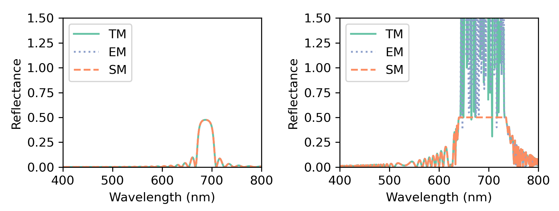
Fig. 5 Reflection spectra calculated with the transfer matrix method (TM and EM) and the scattering matrix method (SM) for chole_1 (left) and chole_2 (right).
With the scattering matrix method (SM), the spectra took about 40 seconds to be calculated on a laptop, against 20 seconds for the transfer matrix method with the eigenvalue and eigenvector calculation (TM) and 35 seconds for the transfer matrix method with the direct exponential of Berreman’s matrix (EM).
The SM method always gives accurate results. However, for speed, the user may prefer using the TM transfer matrix method. The user should always check that the results calculated with TM match these calculated with SM in the most critical conditions of the user’s range of parameters (higher birefringence, larger number of periods, larger angle of incidence).